Predicting status of Tanzanian water pumps

23 Jan 2017

This post is a thorough explanation of my process for creating a model for the “Pump it Up” competition hosted by DrivenData. The model’s classification rate is in the top 4.8% of all submissions according to the leaderboard at the time of this writing.

The problem

Our objective is to predict the status of Tanzanian water pumps. The water pumps are either functional, non-functional, or they are functional but need repair. We are given 40 predictor variables which range from the gps location of the pumps to the quality and quantity of water of each pump, among other interesting metrics. More information about the problem and the variables can be found on this page. This is a pretty standard multi-class classification problem.

Exploratory data analysis

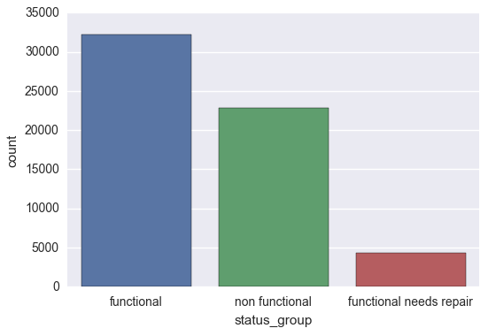
We begin our exploration by taking a glance at the target variable. From the output below, we can see that we are dealing with unbalanced classes, particularly in the case of the ‘functional needs repair’ pumps.

sns.countplot(y_train['status_group'])

The main goal of our exploratory analysis is to identify the type, the quality, and the variability of our input variables. Let us begin with the following command:

for i in X_train.columns:
    print i,',' ,'{:.1%}'.format(np.mean(X_train[i].isnull())),'nulls',',',type(X_train[i][0]), 
    X_train[i].nunique(), 'unique values'

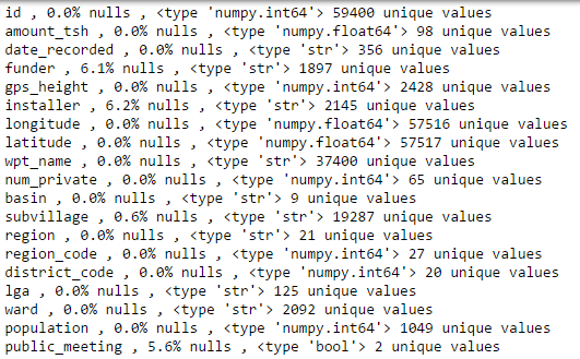
After additional investigations (not necessary to illustrate here, but feel free to consult the Github link noted at the end) our exploratory data analysis leads to several key conclusions that inform the feature engineering:

The majority of the variables are categorical, although we have a handful of numerical features, as well as a couple of temporal features.
We are going to have to address several columns with null values. It bears mentioning that several numerical features show up as being complete in the output above, but upon a closer inspection of their distribution (not shown here), we notice that there are many zeros, which are as good as nulls in this case. Therefore, imputation will be a key factor in our feature engineering.
Several categorical variables have a very large number of unique values. During our feature ranking process, we will have to decide what to do with low-frequency values.
A cross-tab inspection reveals that there are multiple examples of redundant features that more or less contain the same data. A good example of this is quantity and quantity_group.

Feature engineering

The majority of time for this project was spent in feature engineering. In this section, I will present and explain all the essential helper functions that prepared the data for the model.

Continuous variables imputation

For longitude, latitude, gps_height, and population, we can estimate the null and zero values by taking their mean within each district_code or basin and using those values to fill in the missing ones. This technique should give us a more accurate estimate than merely taking the overall average. Additionally, we will take the log of population, although generally speaking the scale of a variable doesn’t affect a random forest model.

def locs(X_train, X_test):
    trans = ['longitude', 'latitude', 'gps_height', 'population']
    for i in [X_train, X_test]:
        i.loc[i.longitude == 0, 'latitude'] = 0
    for z in trans:
        for i in [X_train, X_test]:
            i[z].replace(0., np.NaN, inplace = True)
            i[z].replace(1., np.NaN, inplace = True)
        
        for j in ['subvillage', 'district_code', 'basin']:
        
            X_train['mean'] = X_train.groupby([j])[z].transform('mean')
            X_train[z] = X_train[z].fillna(X_train['mean'])
            o = X_train.groupby([j])[z].mean()
            fill = pd.merge(X_test, pd.DataFrame(o), left_on=[j], right_index=True, how='left').iloc[:,-1]
            X_test[z] = X_test[z].fillna(fill)
        
        X_train[z] = X_train[z].fillna(X_train[z].mean())
        X_test[z] = X_test[z].fillna(X_train[z].mean())
        del X_train['mean']
    return X_train, X_test

X_train['population'] = np.log(X_train['population'])
X_test['population'] = np.log(X_test['population'])

Linear discriminant analysis

One of our concerns with this model is its high dimensionality due to the large number of dummy variables that are created once the categorical columns are converted to integers. Thus, we want to implement dimensionality reduction techniques whenever possible, and our continuous variables longitude, latitude, and gps_height are excellent candidates for linear discriminant analysis. The function below allows us to do that.

def lda(X_train, X_test, y_train, cols=['gps_height', 'latitude', 'longitude']):
    sc = StandardScaler()
    X_train_std = sc.fit_transform(X_train[cols])
    X_test_std = sc.transform(X_test[cols])
    lda = LDA(n_components=None)
    X_train_lda = lda.fit_transform(X_train_std, y_train.values.ravel())
    X_test_lda = lda.transform(X_test_std)
    X_train = pd.concat((pd.DataFrame(X_train_lda), X_train), axis=1)
    X_test = pd.concat((pd.DataFrame(X_test_lda), X_test), axis=1)
    for i in cols:
        del X_train[i]
        del X_test[i]
    return X_train, X_test

Date columns

In our first piece of feature extraction, we create year_recorded and month_recorded columns and convert them into dummy variables (the process is broken into two functions for testing between keeping the columns as numerical vs. categorical). We keep the date_recorded column, but we convert to an ordinal so that our model has an easier time interpreting it.

def dates(X_train, X_test):

    for i in [X_train, X_test]:
        i['date_recorded'] = pd.to_datetime(i['date_recorded'])
        i['year_recorded'] = i['date_recorded'].apply(lambda x: x.year)
        i['month_recorded'] = i['date_recorded'].apply(lambda x: x.month)
        i['date_recorded'] = (pd.to_datetime(i['date_recorded'])).apply(lambda x: x.toordinal())
    return X_train, X_test

def dates2(X_train, X_test):
    """
    Turn year_recorded and month_recorded into dummy variables
    """
    for z in ['month_recorded', 'year_recorded']:
        X_train[z] = X_train[z].apply(lambda x: str(x))
        X_test[z] = X_test[z].apply(lambda x: str(x))
        good_cols = [z+'_'+i for i in X_train[z].unique() if i in X_test[z].unique()]
        X_train = pd.concat((X_train, pd.get_dummies(X_train[z], prefix = z)[good_cols]), axis = 1)
        X_test = pd.concat((X_test, pd.get_dummies(X_test[z], prefix = z)[good_cols]), axis = 1)
        del X_test[z]
        del X_train[z]
    return X_train, X_test

Construction year column

The construction_year column has 35% nulls (or rather, zeros), so we replace those values with the mean of the column

def construction(X_train, X_test):
    for i in [X_train, X_test]:
        i['construction_year'].replace(0, X_train[X_train['construction_year'] <> 0]['construction_year'].mean(), inplace=True)
    return X_train, X_test

Boolean column imputation

The permit and public_meeting columns have 5.1% and 5.6% nulls, respectively. We equate the nulls to False, since we don’t know anything about these columns. For the record, I did try null flag variables, but they proved to be useless.

def bools(X_train, X_test):
    z = ['public_meeting', 'permit']
    for i in z:
        X_train[i].fillna(False, inplace = True)
        X_train[i] = X_train[i].apply(lambda x: float(x))
        X_test[i].fillna(False, inplace = True)
        X_test[i] = X_test[i].apply(lambda x: float(x))
    return X_train, X_test

Feature selection: removing useless columns

Here we define all the columns that we want to delete right off the bat:

id is not a useful predictor
amount_tsh is mostly blank
num_private is ~99% zeros
region is highly correlated with region_code
quantity is highly correlated with quantity_group
quality_group is highly correlated with quality
source_type is highly correlated with source
payment is highly correlated with payment_type
waterpoint_type_group is highly correlated with waterpoint_type
extraction_type_group is highly correlated with extraction_type
scheme_name is almost 50% nulls, so we will delete this column

def removal2(X_train, X_test):
    z = ['id','amount_tsh',  'num_private', 'region', 
          'quantity', 'quality_group', 'source_type', 'payment', 
          'waterpoint_type_group',
         'extraction_type_group']
    for i in z:
        del X_train[i]
        del X_test[i]
    return X_train, X_test

Feature selection: removing low-frequency values

In what amounts to the biggest judgement call of our model, we decide to group low-frequency values in the categorical variables into ‘other’ (for each column). This was a tricky decision because the model where no grouping was done actually performed slightly better than the model with grouping. However, the difference was negligible. Meanwhile, the benefits of doing this are reducing computational cost as well as mitigating overfitting. Even so, we picked a relatively small cutoff value, and it might be better to increase that cutoff to something like 100.

def small_n(X_train, X_test):
    cols = [i for i in X_train.columns if type(X_train[i].iloc[0]) == str]
    X_train[cols] = X_train[cols].where(X_train[cols].apply(lambda x: x.map(x.value_counts())) > 20, "other")
    for column in cols:
        for i in X_test[column].unique():
            if i not in X_train[column].unique():
                X_test[column].replace(i, 'other', inplace=True)
    return X_train, X_test

Dummy variable creation

Last but not least, we convert the remaining categorical variable sinto dummy variables so that they are compatible with sci-kit learn.

def dummies(X_train, X_test):
    columns = [i for i in X_train.columns if type(X_train[i].iloc[0]) == str]
    for column in columns:
        X_train[column].fillna('NULL', inplace = True)
        good_cols = [column+'_'+i for i in X_train[column].unique() if i in X_test[column].unique()]
        X_train = pd.concat((X_train, pd.get_dummies(X_train[column], prefix = column)[good_cols]), axis = 1)
        X_test = pd.concat((X_test, pd.get_dummies(X_test[column], prefix = column)[good_cols]), axis = 1)
        del X_train[column]
        del X_test[column]
    return X_train, X_test

Running the above helper functions results in 2455 predictive variables for us to model.

Other transformations considered

In addition to the above transformations, some of the things I tried but which didn’t have a positive impact on the results were:

imputing the missing construction_year values according to the same methodology as latitude and longitude
varying the cutoff threshold for values that would be grouped into ‘other’ for categorical variables
combining date_recorded and construction_year into a new column that designated length of operation
for each categorical column, combining small-n values based on their propensity to be indicative of functional, non-functional, or in-need of repair
keeping amount_tsh and imputing the missing values

Hyperparameter tuning

In order to tune our hyperparameters, we will use grid search. The main issue with running grid search, of course, is the massive computational cost of doing the brute force calculations. However, tuning the hyperparameters often leads to much-needed performance improvement, so the cost of waiting is generally worth it. One option is to run the gridsearch on only one parameter at a time, thereby significantly reducing the number of permutations that need to occur.

As we have chosen to build a random forest mdoel, the primary parameters we will need to tune are min_samples_split and n_estimators. As the output below shows, the optimal values are 6 for min_samples_split and 1000 for n_estimators.

rf = RandomForestClassifier(criterion='gini',
                                n_estimators=500,
                                max_features='auto',
                                oob_score=True,
                                random_state=1,
                                n_jobs=-1)

param_grid = {"min_samples_split" : [4, 6, 8],
             "n_estimators" : [500, 700, 1000]}

gs = GridSearchCV(estimator=rf,
                  param_grid=param_grid,
                  scoring='accuracy',
                  cv=2,
                  n_jobs=-1)

gs = gs.fit(X_train, y_train.values.ravel())

print(gs.best_score_)
print(gs.best_params_)
print(gs.grid_scores_)

Model execution and evaluation

After running the model with the optimal hyperparameters, we get an out-of-bag score or 0.8134. Although this is supposed to be an unbiased estimate of the classification rate, when we do cross-validation, we get a score of 0.8071, which is actually lower than our test score (from the actual leaderboard) of 0.8181.

rf32 = RandomForestClassifier(criterion='gini',
                                min_samples_split=6,
                                n_estimators=1000,
                                max_features='auto',
                                oob_score=True,
                                random_state=1,
                                n_jobs=-1)
                            
rf32.fit(X_train, y_train.values.ravel())
print "%.4f" % rf32.oob_score_

Note that we choose stratified k-fold cross-validation because our classes are not balanced.

kfold = StratifiedKFold(y=y_train.values.ravel(), n_folds=3, random_state=1)
scores = []
for k, (train, test) in enumerate(kfold):
    rf3.fit(X_train.values[train], y_train.values.ravel()[train])
    score = rf3.score(X_train.values[test], y_train.values.ravel()[test])
    scores.append(score)
    print('Fold: %s, Class dist.: %s, Acc: %.3f' % (k+1, np.array(y_train['status_group'][train].value_counts()), score))

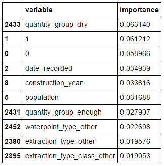
Looking at the variable importance, we can see that our two linear discriminants 0 and 1 are in the top three most important variables. The one surprise here is that their expected orders of importance are reversed.

pd.concat((pd.DataFrame(X_train.columns, columns = ['variable']), 
           pd.DataFrame(rf32.feature_importances_, columns = ['importance'])), 
          axis = 1).sort_values(by='importance', ascending = False)[:10]

Concluding remarks

This model was a relatively straightforward model, although I definitely explored a lot of different variations before arriving at this one. One potentially negative advantage of competitions is the ability to make multiple submissions. Although this allows us to test many different models and learn a lot, it does also mean that we are in danger of overfitting our model to the test data, therefore resulting in an inflated measure of model accuracy.

All of the code from this analysis can be found on my Github page:
https://github.com/zlatankr/Projects/tree/master/Tanzania

Feel free to comment and/or message me with suggestions, comments, or corrections.