Bayesian A/B testing with Thompson sampling

07 Apr 2017

In this academic module, we will explore the theory behind the Bayesian approach to A/B testing. This approach has recently gained traction and in some cases is beginning to supersede the prevailing frequentist methods. After laying down our theory, we will take a look at a practical example.

Frequentist statistics

Frequentist statistics centers around the (now) traditional approach of collecting data in order to test a hypothesis. Frequentist inference relies on these steps:

Formulate a hypothesis.
Collect the data.
Calculate essential test statistics, including p-value and confidence intervals.
Decide whether or not to reject the null hypothesis.

The important assumption in frequentist statistics is that the parameters of a distribution are set, but we do not know what they are. The data we then collect is a function of those parameters and the underlying distribution. Mathematically, we can express this as:

\begin{align} \hat \theta = argmax_\theta P(X \mid \theta) \end{align}

where X is our data sample, θ is the underlying distribution of the data under the null hypothesis, and θ-hat is the observed parameter.

This approach is very useful in drawing conclusions about data from scientific studies and any other hypotheses, and the use of confidence intervals provides a very intuitive way of understanding our observed parameters. However, the frequentist approach does have several drawbacks, including:

stopping a test early when we see a significant p-value increases our chances of getting a false positive.
we are not able to measure the probability that our conclusion in the study is true.
p-values are prone to misinterpretation.
experiments must be fully specified ahead of time, which can lead to paradoxical seeming results.

Multi-armed bandit problem

Before we jump into Bayesian inference, it is important to contextualize our problem with a useful (and classic) scenario. In the multi-armed bandit problem, we are at a casino (hence ‘bandit’) playing slot machines (hence ‘armed’). Given that not all slot machines have the same payout, if we are playing two slots, then we are going to start seeing different results from the two machines. This leads to the ‘explore vs. exploit dilemma,’ where we are forced to decide between exploiting the higher-payout machine and exploring the options (at random) in order to collect more data. To any degree that we choose to exploit, we are adapting our behavior to the observed data, and this is one of the general premises behind reinforcement learning. Our goal is to maximize our reward and minimize our loss by increasing our certainty that we are making the right decision.

There are several strategies one can use to approach the multi-armed bandit problem, including using the Epsilon-Greedy or the UCB1 algorithm, but this is also where Bayesian inference comes in.

Bayesian statistics

Bayesian statistics revolve around, oddly enough, Bayes’ theorem, which states that the conditional probability of A given B is equal to the conditional probability of B given A times the probability of A divided by the probability of B:

\begin{align} \ P(A \mid B) = \frac{P(B \mid A)P(A)}{P(B)} \end{align}

In our scientific problem of trying to draw a conclusion about a parameter given a set of data, we can now treat that parameter as a random variable that has its own distribution, thus giving us:

\begin{align} \ P(\theta \mid X) = \frac{P(X \mid \theta)P(\theta)}{P(X)} \end{align}

Here,

P(θ|X) is known as the posterior, meaning our new beliefs about our parameter in question, θ, given our data X.
P(X|θ) is known as the likelihood, anwsering the question of how likely is our data given our current θ.
P(θ) is the prior, meaning our old beliefs about θ.
P(X) is the integral over P(X|θ)P(θ)dθ, but because it doesn’t contain θ, it can be ignored as a normalizing constant.

Now we can see the Bayesian paradigm shift. Unlike the frequentist method, here we take into account the distribution of our parameter both before and after the collecting the data. Knowing the distribution of our parameter will allow us to assign a given confidence to our estimate of that parameter.

But how do we know the probability distribution of our posterior? The answer lies in the concept of the ‘conjugate priors,’ which states that if the prior probability distributions are in the same family as the posterior distributions, then they are known as conjugate distributions, and the prior is known as the conjugate prior to the likelihood function. In simpler terms, if we know the distribution of the likelihood function, we can determine the distribution of the posterior and prior.

As an example, let’s assume that we are measuring a click-through rate (whether somebody clicks on an advertisement or not). Because we are measuring a binary outcome (did somebody click on or not), we know that we are dealing with the Bernoulli distribution, making our likelihood:

\begin{align} \large P(X \mid\theta) = \prod_{i=1}^N \theta^{x_i}(1-\theta)^{1-x_i} \end{align}

The conjugate prior to the Bernoulli distribution is the Beta distribution:

\begin{align} \theta \sim Beta(a,b) = \frac{\theta^{a-1}(1-\theta)^{b-1}}{B(a,b)} \end{align}

where B(a,b) is the Beta function.

If we try to solve for the posterior, first we would combine the likelihood and the prior:

\begin{align} \large P(\theta \mid X) \propto \prod_{i=1}^N \theta^{x_i}(1-\theta)^{1-x_i}\theta^{a-1}(1-\theta)^{b-1} \end{align}

This would simplify into:

\begin{align} \large P(\theta \mid X) \propto \theta^{a-1+\sum_{i=1}^Nx_i}(1-\theta)^{b-1+\sum_{i=1}^N(1-x_i)} \end{align}

Thus, we can see that P(θ|X) does in fact have a Beta distribution, but with slightly modified hyperparameters. Let’s look a little closer. We can conclude that

\begin{align} \ P(\theta \mid X) = Beta(a’,b’) \end{align}

where

\begin{align} \ a’ = a+\sum_{i=1}^Nx_i,\text{ }b’ = b+N -\sum_{i=1}^Nx_i \end{align}

or, in terms of our click-through rate problem, a’ = a + #(clicks), b’ = b + #(no clicks).

Intuitively, this makes sense because it tells us that our posterior distribution is a function of our collected data, and additionally, the posterior distribution could then be used as the prior for more samples, with the hyperparameters simply adding each extra piece of information as it comes.

Taking a further look at the Beta distribution, we note that the mean of the distribution is:

\begin{align} \ E(\theta) = \frac{a}{a+b}, \end{align}

which is the same as what we would have gotten had we maximized the likelihood. Lastly, the variance of the Beta distribution decreases as a and b increase, which is analogous to the behavior of confidence intervals with the frequentist approach.

\begin{align} \ var(\theta) = \frac{ab}{(a+b)^2(a+b+1)} \end{align}

Example: Thompson sampling

In this example we will demonstrate how the multi-armed bandit problem is solved with Bayesian inference using Thompson sampling. We will use 2,000 trials and our three bandits will have underlying payout probabilities of .2, .5, and .75. First, we define a bandit class that has a given probability. The class with have a method that returns a reward or loss (1 or 0) based on its probability. We will also be able to update its a and b values and use those values to sample from the resulting Beta distribution.

import matplotlib.pyplot as plt
import numpy as np
from scipy.stats import beta


NUM_TRIALS = 2000
BANDIT_PROBABILITIES = [0.2, 0.5, 0.75]

class Bandit(object):
  def __init__(self, p):
    self.p = p
    self.a = 1
    self.b = 1

  def pull(self):
    return np.random.random() < self.p

  def sample(self):
    return np.random.beta(self.a, self.b)

  def update(self, x):
    self.a += x
    self.b += 1 - x

Next, we will define a function to plot the Beta distribution of our bandits.

def plot(bandits, trial):
  x = np.linspace(0, 1, 200)
  for b in bandits:
    y = beta.pdf(x, b.a, b.b)
    plt.plot(x, y, label="real p: %.4f" % b.p)
  plt.title("Bandit distributions after %s trials" % trial)
  plt.legend()
  plt.show()

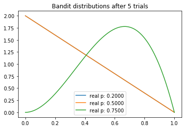
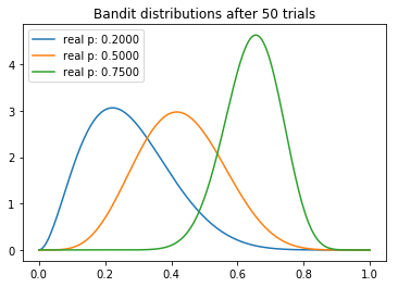
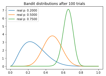
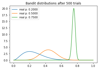
Now, onto our experiment. First, we initialize each of our three bandits. We will plot their distributions at our predetermined sample_points. For each trial, we will sample from each bandit’s distribution and pick the bandit with the highest probability of a payout. The winning bandit will then have a chance to pull its hand and consequently update its a and b values.

def experiment():
  bandits = [Bandit(p) for p in BANDIT_PROBABILITIES]

  sample_points = [5,50,100,500,1999]
  for i in xrange(NUM_TRIALS):

    # take a sample from each bandit
    bestb = None
    maxsample = -1
    allsamples = [] # let's collect these just to print for debugging
    for b in bandits:
      sample = b.sample()
      allsamples.append("%.4f" % sample)
      if sample > maxsample:
        maxsample = sample
        bestb = b
    if i in sample_points:
      print "current samples: %s" % allsamples
      plot(bandits, i)

    # pull the arm for the bandit with the largest sample
    x = bestb.pull()

    # update the distribution for the bandit whose arm we just pulled
    bestb.update(x)

Let’s run the experiment and see what happens.

experiment()

current samples: ['0.2031', '0.8931', '0.8184']

current samples: ['0.1958', '0.4464', '0.6787']

current samples: ['0.3299', '0.5376', '0.7011']

current samples: ['0.2830', '0.4962', '0.7628']

current samples: ['0.3545', '0.3741', '0.7555']

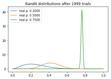
We can make several interesting observations about our experiment. We note that the mean of each distribution gradually converges around its true value. But we can see that the highest-payout bandit has the lowest variance, which is a reflection of the fact that it has the highest N. However, this is not necessarily a problem, because the by the end there is almost no overlap between the highest distribution and the two lower ones, meaning that the probability that sampling from the inferior bandits would yield a higher payout is minimal (as can be seen by the ‘current samples’ printout).

Probability of results

Another benefit of the Bayesian inference with Thompson sampling is that we can calculate the probability that a given result is better than its alternative. For example, if we are measuring click-through rates of two competing pages, our expected payout would be the mean of our posterior distributions. Then, probability that a given mean is higher than another can be calculated as the area under their join probability distribution function where mean two is higher than mean one:

\begin{align} \ P(\mu_2 > \mu_1) = \text{area under } p(\mu_2, \mu_1) \text{ where } \mu_2 > \mu_1 \end{align}

Mathematically, we can calculate this as:

\begin{align} \ P(\mu_2 > \mu_1 = \displaystyle \sum_{i=0}^{a_2-1} \frac{B(a_1+i,b_1+b_2)}{(b_2+1)B(1+i,b_2)B(a_1,B_1)} \end{align}

Conclusion

As with most battles between intellectually viable sides, there is usually no clear winner. And so it is with Bayesian and frequentist methodologies. Both offer their own interesting solutions to the problem of A/B testing, and it is best to first evaluate the scenario before choosing an approach. The last link in the references below offers some good tips as to when bandit tests (which include our Thomspon sampling) are applicable.

References: